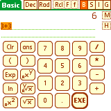
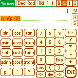

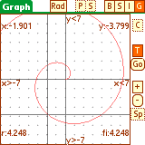


EasyCalc is a scientific graphing calculator for PalmOS devices. It has the ease-of-use of the built-in PalmOS Calculator, but adds all the features of a top-of-the-line (TI-89, HP-49) scientific graphing calculator except CAS (computer algebra system) and programming (although user defined functions are possible).
This manual is based on the EasyCalc documentation submitted by <halliday at users.sourceforge.net> and Ondrej Palkovsky's tutorial from previous EasyCalc versions. It also covers the new features introduced in recent versions (>= 1.23).
Features and Specifications:
Back to Contents
Using the Palm Install program, install the files 'MathLib.prc' and one of the other 'calc_*.prc' files. They are all language-localized versions (Czech, German, English, French, Italian, Japanese, Portuguese, Russian, and Spanish). 'calc_small.prc' (104K) is a non-graphing scientific calculator in English, with none of the special functions.
If needed import your user variables and functions from Memopad.
Note that on newer devices (e.g. T|X, Treo 650/680/700p) MathLib is already
installed as part of the system software. If you are not sure just install
EasyCalc without MathLib and start it.

If you do not get the alert that MathLib is needed you are OK.
Simply delete the 'Easy Calc' application. If you have no other programs that require MathLib, you may remove that as well.
See also the file INSTALL in the distribution which contains the most recent information about installing EasyCalc.
Back to Contents
To enter numbers or functional expression (such as 3*sin(pi/2)), you may use the on-screen buttons, graffiti and/or keyboard, and switch between them at will.
EasyCalc supports 'implicit' multiplication (without the '*' operator):
3e+1
ans> 9.154 845 485
3E+1
ans> 30
The priority of the hidden implicit multiplication operator is very
high. When you enter 3^6pi, 3^(6*pi) is executed.
The priority of an explicitly written multiplication '*' operator is as
expected.
EasyCalc doesn't require closing parentheses:
2sin(pi/2
...is interpreted as 2*sin(pi/2)
ans>2
The 'ANS' button displays the last computed result.
The 'ans' variable is inserted automatically when you are at the
beginning of the line, and press some 'operation' button.
Example:
sin(pi)
...now tap the 'plus' button
ans> ans+
...now complete the expression with '1', and tap EXE to compute sin(pi)+1>.
Tip: if you select an expression (or a part of it), and then tap a
function button, the selected text is inserted into the function and
remains selected.
This works for parentheses, too: if you forgot to put part of an
expression in parens, simply select it and tap the '(' button.
On the main EasyCalc screen:
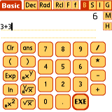
The first line below the menu bar is the 'Results Line', where EasyCalc
displays the results of computations or error messages.
If the contents of the Result Line are too long to display, tap and drag
the Result Line left and right to see the whole thing.
The next two dotted lines are the 'Entry Line', where user input is entered.
On the top line of the main screen:
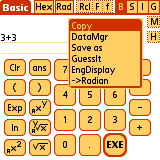
The 'Special' menu allows access to the Data Manager, Financial Manager, List Editor, Matrix Editor, and Solver.
Back to Contents
EasyCalc supports all common (and most uncommon) mathematical functions and operations found on the best scientific calculators. See the Function Reference sections for a complete list of all functions.
Two basic calculator layouts are available by tapping 'B' at the top of the screen. Use the Preference screen to choose which basic layout to use.
EasyCalc supports an unlimited number of variables and functions. Variable names cannot be: pi, e, f, i, j, k, m, n, p, u, or x (see the Function Reference section for details). They may consist of lower-case letters, numbers, and the underscore symbol '_', and can be up to 10 characters long. If you define a variable with the same name as a function, the function will be overwritten (and vice versa).
A variable is defined by entering:
name=value
Example:
a=31
The value 31 is stored in variable 'a', which can be used in other
expressions and calculations.
If you then enter a=3*a thevariable 'a' will contain the number 93.
A function is defined by entering:
name()="expression"
The "expression" must be enclosed in double quotes, and the
parentheses must be left empty).
Example:
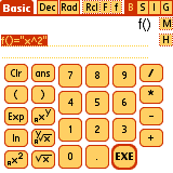
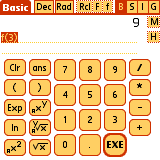
f()="x^2"
f(3)
ans> 9
Function definitions must use 'x' as the parameter.
You can delete or edit defined functions and variables by tapping the
'DataMgr' in the 'M'-menu (to the right of the Result Line).
To define functions that accept more then one input variable, use 'x' or 'x(1)' for the first parameter, 'x(2)' for the second parameter, 'x(3)' for the third, etc. When calling the function, separate values with a colon.
Example (quadratic formula):
quadsoln1()="( -x(2) + sqrt(x(2)^2 - 4*x(1)*x(3)) ) / (2*x(1))"
quadsoln1(1:-2:-3)
ans> 3
You can separate multiple expressions or definitions on one line with a semicolon ';'. Only the result of the last expression is displayed.
Example:
a=3;b=7;c=4;quadsoln1(a:b:c)
ans> -1
b^2
ans> 49
EasyCalc can't execute 'programs', except by separating functions and expressions with the semicolon.
EasyCalc can save its workspace of user-defined variables and functions to MemoPad. In the Special menu, select 'Export to memopad' or 'Import from memopad'. If there is a category named 'EasyCalc' in MemoPad, only memos from that category are displayed.
The first line of an imported memo (the title) is not executed. The imported memo is executed just as if you inserted the text line-by-line into the calculator.
Simple function routines can be built using the semicolon, lists for input/output series, user defined variables and functions, and the ask(), and if() functions, although only one line can be executed at a time.
ask("title"{:default value}) - opens a dialog with the (optional) default entered. Returns the user input.
if(test:true-expr:false-expr) - evaluates test and returns the appropriate expression. Test must return a positive integer ('true') or zero ('false'). The not used expression is not evaluated.
Example: Recursive factorial definition.
myfact(x)="if(x>1:x*myfact(x-1):1)"
ans> myfact()
myfact(3)
ans> 6
myfact(100)
ans> Too deep recursion - Limited stack space for recursion !!!
res=myfact(ask("Enter argument for myfact":5))
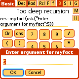
Tap/Select 'OK'
ans> 120
EasyCalc can rationalize a number to fractions, common square roots, and powers of e or pi. If the number is integer it tries to write the number as prime factors
Examples:
acos(0)
ans> 1.570 796 327
in the 'M' menu, choose 'GuessIt':
ans> pi/2
6/21+1/5
ans> 0.485 714 286
'M' ->GuessIt
ans> 17/35
533
ans> 533
'M' ->GuessIt
ans> 13*41
Back to Contents

Radian/Degree/Grad mode - applies to all calculations. Can also be set on the main screen.
Decimal/Binary/Octal/Hexadecimal - sets output formatting mode. Can also be set on the main screen.
Normal/Scientific/Engineer - display mode for results.
Scientific Calc in Basic Mode - Allows you to choose between two layouts of the Basic screen - either very basic, or with some scientific functions (and more crowded).
Force integer nums - Note: Graphing will NOT work properly with this checked. Generally, you will not check this UNLESS you are working with base conversions. This setting applies to input recognition and displaying results, but doesn't change computing behavior. The expression '3.14159' isn't recognized in integer modes (Bin/Oct/Hex), because '3.14159' is a floating point number. 'pi' outputs the correct result regardless of mode, because 'pi' is a floating point constant. Floating point output formatting prints at most 10 digits, but integer number formatting will print always the whole number - this makes sense only for 32-bit numbers converted to Binary. See the Integer/Base Operations section for more details.
Precision - the number of digits to display after the decimal point.
Reduce precision - When checked, floating point numbers are rounded off to 11 places after each calculation, and will round certain results smaller than 1E-14 to zero. This avoids results like: sin(pi)=1E-15. Selecting this option slows all operations a little, so I recommend switching it off if you are going to use Numerical Analysis (fzero(), etc.). If you use Numerical Analysis in Graphing mode, 'Reduce precision' turns off automatically.
Strip zeros - output '3.100' or '3.1'
Insert Help - insert argument names for some multiparameter functions on the input line.
Match ()'s - Can be very handy. If checked, then tapping a function button automatically inserts the closing bracket and moves the cursor position between the brackets.
Palm Num Prefs - If checked, EasyCalc allows entering numbers exactly according to PalmOS Preferences. Not recommended unless you use clipboard for moving data from other applications.
Show Units - If checked and the engineer mode is selected, numbers get a unit to them at the output (e.g. 1E6 -> 1M ).
Back to Contents
Switch to Graph mode by tapping the 'G' at the top of the screen (or 'Menu->Layout->Graph').
Set up the functions to graph by tapping 'S' (or 'Menu-> Graph-> Setup funcs').

Tap the area to the RIGHT of 'Y1' and enter any valid expression in terms
of 'x', such as 'x^2-4' - but WITHOUT any quotes.
For each graph you can select the color and the line style
(line/points/vertical). Each graph can be turned on and off individually.
The color of the axes, the grid and the graph background are also user
selectable. You can also turn the axes, axes labels and the grid on and off.
Change Graph Preferences by tapping 'P' (or 'Menu -> Graph
-> Preferences').
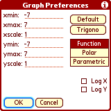
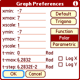
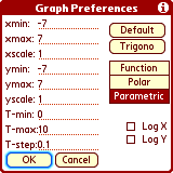
Here you can setup the display area (min and max bounds, grid interval) and
type of graph (normal, polar, parametric). Either axis can be logarithmically
scaled. Note that for Polar graphs the angle units (t-min, t-max, t-step)
obey the Rad/Deg/Grd setting.
You may also enter an existing user-defined function, and if necessary, pass it additional parameters (to make it a graphable function of one variable).
Example:
In Scientific mode, define this familiar function of 1 variable 'x', and
3 other parameters:
quad()="x(2)*x^2 + x(3)*x + x(4)"
In Graphing mode,
Tap 'S' to Setup Graphs.
Tap the area to the right of 'Y1'.
Tap 'F' (user functions) and select quad().
Enter 4 parameters for quad(), which will be passed to x, x(2), x(3),
and x(4). Here, we tell EasyCalc to take the first parameter as the
independent variable for the graph (must always be 'x'), and take the
other three as constant parameters:
quad(x:1:-2:-3)
You may enter up to six functions in each mode (Function, Polar,
Parametric). The functions are stored as 'z_grafun1()', 'z_grapol1()',
'z_grapara1()', etc., and can be
used and modified in the non graphical modes.
When entering an expression, the 'Rcl', 'F', and 'f' buttons are
available and work the same as on the main screen.
To remove a function, tap the 'Y1' button itself and select 'Delete' from
the popup menu.
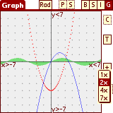
To trade graphing speed for resolution and accuracy, tap the 'Sp' button
to set the speed. Is speed 'n' is selected only every n-th point is plotted.
You can see this clearly if you select the points linestyle.
Tap and drag the graph to scroll around.
'-' button - zoom out
'+' button - zoom in. Tap '+' and then draw a zoom area on the graph.
(Menu-> Graph-> Table Mode) displays exact values of the parameter 'x'
and values of all the functions simultaneously.
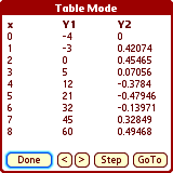
GoTo will start the table at a specific value (Tip: you may just write a
number, without tapping GoTo first)
The initial table step value is set by the 'xscale' parameter in Graph
Preferences. It can be changed on the Table Mode form by tapping the Step
button.
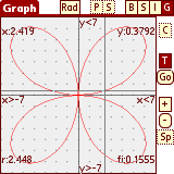
EasyCalc can find a zero (root), value, local minimum and maximum of a
function, first and second derivatives, integral, and intercept with
another function:
Tap the 'C' button.
Select an operation.
Select a function.
You will be instructed to enter the left and right bounds (for zero,
min, max, intercept), or the point to calculate at (for derivatives &
integral). Tap OK to dismiss the instructions, then locate the point,
and then tap 'C' again to confirm the entry.
For intercept, you will now select a second function.
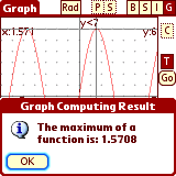
The result of the operation will be stored in a variable called 'graphres'.
Back to Contents
Normal, inverse, and hyperbolic trig functions work as expected. See the Function Reference for a complete list.
Trig functions can take complex, list, or matrix arguments. For lists and matrices, the function is applied to each element individually.
Set Deg/Rad/Grad mode by tapping the indicator at the top of the screen,
or in Menu->Preferences.
Note: Be sure to check the mode when using Trig functions!
Trig display conversions are found in the 'M' menu (on the right side of
the Results Line):
M ->GuessIt - may come up with a helpful simplification
in Deg mode:
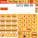

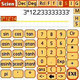
M ->Degree - display as D°M'S
M ->Degree2 - display as D°M.sss'
in Rad mode:
M ->Radian - displays result as a multiple of pi
The following results depend on the Deg/Rad/Grad setting. The mode is set to Degree for the examples.
Rectangular to Polar:
rtopr(x:y) - Radius of the point (x,y)
rtopd(x:y) - Angle of the point (x,y)
rtop(x:y) - Returns a list [radius:angle].
Polar to Rectangular:
ptorx(rad:ang) - x-coord of point at radius, angle
ptory(rad:ang) - y-coord of point at radius, angle
ptor(rad:ang) - returns a list [x:y].
hypot(x:y) - returns the length of the hypotenuse of a right triangle
with sides x and y.
Examples (in Deg):
rtopr(1:sqrt(3))
ans> 2
ptor(2:30)
ans> [1.732050808:1]
hypot(1:1)
ans> 1.414 213 562
Example(in Rad Mode):
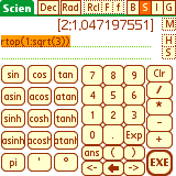
rtop(1:sqrt(3))
ans> [2:1.047197551]
Back to Contents
Lists are defined in the form:
[1:2:3]
Matrices with m(rows) x n(cols) are defined in the form:
[[1:2:3]:[3:4:5]]
...this operation creates 2 by 3 matrix that is stored in the variable
'ans'.
Lists/Matrices can be stored to a variable directly from the Input Line:
d=[[1.1:-2.2:3]:[1:1.4:4]:[6:1.5:-2.6]]
list1=[1:-2:2:3:0:4:-4:0:7:5]
Lists/matrices too large to be displayed entirely on the results line
will show only their dimensions:
ans> list(..20..)
ans> matrix(8,3)
Tapping the Result Line when it contains a list or matrix takes you into
the List or Matrix Editor. The List and Matrix Editors can also be
accessed from the 'Special' menu.
In the List/Matrix Editors, you specify the name for the list/matrix,
its dimensions, and the values of the elements. If necessary, scroll
using the arrows at the bottom and/or right of the screen.
Tip: in the List Editor, once a list has been selected for editing, you can just start writing to append elements to the end.
If a scalar variable or a function is entered into a list or matrix, it is pre-evaluated. Only the value, not the variable reference, is stored in the matrix. Also, a matrix can be built from lists of the appropriate size.
Example:
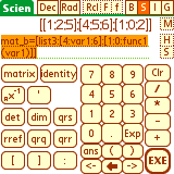
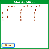
func1()="x-3"
var1=5
list3=[1:2:var1]
mat_b=[list3:[4:var1:6]:[1:0:func1(var1)]]
ans> [[1:2:5]:[4:5:6]:[1:0:2]]
Complex numbers are allowed in lists and matrices:
mat_c=[[1:i+6]:[4i:3]]
dim(x) - dimension (size) of list/matrix 'x'. Returns a scalar if the
input is a list, and a list if the input is a matrix:
dim([1:2:3:-1])
ans> 4
dim([[1:2:3]:[3:4:5]])
ans> [2:3]
list(elem{:elements}) - returns a list composed of the elements. If the
elements are lists themselves, list() returns a matrix:
list(1:2:3)
ans> [1:2:3]
list([1]:[2:3:4:5])
ans> [[1:0:0:0]:[2:3:4:5]]
matrix(m:n:{elements}) - returns an m x n matrix of elements:
matrix(2:3:1:2:3:4:5:6)
ans> [[1:2:3]:[4:5:6]]
s=list[i] (or list[i:i]) returns the i-th element of a
list
l=list[i:k] (k != i) returns a list with the elements from i to k
of a list
s=matrix[m:n] returns the element of the m-th row and n-th column
of matrix
l=matrix[m:.] (or matrix[m:0]) returns a list with the m-th
row of matrix
l=matrix[.:n] (or matrix[0:n]) returns a list with the n-th
column of matrix
list[i]=val (or list[i:i]=val) assigns val to the i-th
element of list and returns list
list[i:k]=list2 (k != i) assigns the elements of list2 to the
elements from i to k of list and returns list
matrix[m:n]=val assigns val to the (m,n) element of matrix and
returns matrix
matrix[m:.]=list (or matrix[m:0]=list) assigns the elements
of list to the m-th row of matrix and returns matrix
matrix[.:n]=list (or matrix[0:n]=list) assigns the elements
of list to the n-th column of matrix and returns matrix
List addition, subtraction, and multiplication act on elements taken as pairs, so the lists must be of the same size (dimension).
Most scalar functions can take a matrix or list as a parameter, and
return a matrix/list with the function applied to each element:
sin([[pi:0]:[pi/2:3pi/2]])
ans> [[0:0]:[1:-1]]
[1:-2:2:3]^2
ans> [1:4:4:9]
[[1:1]:[2:2]]+1
ans> [[2:2]:[3:3]]
sift(f:x) - drops all elements for which f returns zero
sift("x<9":list(2:9:3:10:1))
ans> [2:3:1]
sift("isprime(x)":range(100))
ans> ..list(xx).. returns list of primes.
sift(x:y) - drops all elements from y where x is zero, both
lists must have same length.
sift(list(1:2:0:1):list(9:2:3:9))
ans> [9:2:9]
find(f:x) - returns indices where f(x) is nonzero.
find("isprime(x)":[10:11:12:13:14])
ans> [2:4] since 11 and 13 are prime.
sample(x:y) - returns the elements of x indexed by y.
sample([0:1:2:3:4]:[1:3:5])
ans> [0:2:4]
map(f:x) - applies f to each element of x.
In most cases this is done transparently:
map("x+1":[3:4])
ans> [4:5]
but in some cases not:
a=list(1:2:3);map("a[x]":list(3:1))
ans> [3:1] (=list(a[3]:a[1])).
map(f:x:y) - applies f to each pair of x and y (not only
matching pairs).
map("x(1)+x(2)":[2:5]:[10:30])
ans> [12:15:32:35]
zip(f:x:y) - applies f to each maching pair of x and y.
zip("x(1)+x(2)":[2:5]:[10:30])
ans> [12:35]
concat(x:y) - concatenates two lists.
concat([1:2]:[3:4:5])
ans> [1:2:3:4:5]
repeat(x:a:b) - will repeat a list's elements. a means how
often to repeat, b means how large parts (0 for full list) to repeat.
repeat([1:2:3:4]:3:0)
ans> [1:2:3:4:1:2:3:4:1:2:3:4]
repeat([1:2:3:4]:3:1)
ans> [1:1:1:2:2:2:3:3:3:4:4:4]
repeat([1:2:3:4]:3:2)
ans> [1:2:1:2:1:2:3:4:3:4:3:4]
repeat([1:2:3:4]:3:3)
ans> [1:2:3:1:2:3:1:2:3:4:4:4]
kron(x:y) - computes all possible products between the elements
of x and those of y.
kron([1:2:3:4]:[1:0:-1])
ans> [1:0:-1:2:0:-2:3:0:-3:4:0:-4]
Back to Contents
Lists are used to store sets of data for statistical analysis.
rand - returns a pseudo-random number between 0 and 1.
rand(n) - returns an n-dimension list containing 'n' pseudo-random
numbers, each uniformly distributed between 0 and 1.
rNorm(n)- returns an n-dimension list containing 'n' pseudo-random
numbers, normally distributed with a mean of 0 and std dev of 1.
range(n{:start{:step}}) - returns an n-dimension list containing
sequential values. Start and step (optional) default to 1.
Examples:
range(4)
ans> [1:2:3:4]
range(4:100)
ans> [100:101:102:103]
range(6:2:3)
ans> [2:5:8:11:14:17]
In the following examples list1=[1:-2:2:3:0:4:-4:0:7:5]
sum(listx) - sum of all elements:
sum([i:1:2])
ans>3+i
cumsum(listx) - list containing the cumulative sum of the
elements:
cumsum(list1)
ans>[1:-1:1:4:4:8:4:4:11:16]
prod(listx) - product of all elements:
prod[1:2:3]
ans>6
mean(listx) - mean of the list computed as sum(listx)/dim(listx):
mean(list1)
ans>1.6
gmean(listx) - geometric mean of the list computed as
prod(listx)^(1/dim(listx)):
gmean(list1)
ans>0
gmean([3:2:5:1])
ans>2.340 347 319
median(listx) - median of the list:
median(list1)
ans>1.5
sorta(listx) - ascending sort
sortd(listx) - descending sort:
sorta(list1)
ans>[-4:-2:0:0:1:2:3:4:5:7]
sortd(list1)
ans>[7:5:4:3:2:1:0:0:-2:-4]
lmin(listx) - minimum value in list
lmax(listx) - maximum value in list:
lmin(list1)
ans>-4
lmax([1:10i:6])
ans>6
lmax(abs([1:10i:6]))
ans>10
lmode(listx) - most frequently occurring item in a list:
lmode([1:2:3:3])
ans>3
The 'unbiased' (Sample) variance is defined as
variance = sum(x-mean(listx)) / (dim(listx)-1).
However, the 'biased' (Population) variance of a list is defined as
variance = sum(x-sum(listx)/dim(listx)) / dim(listx).
variance(listx) or variance(listx:0) - sample variance of
list
variance(listx:1) - population variance
stddev(listx{:flag}) - computes standard deviation where stddev = sqrt(variance()). Uses the variance formula based on the optional flag setting (see variance).
moment(listx:n) - the n'th moment of a list
skewness(listx) - skewness of listx
kurtosis(listx) - kurtosis of listx
varcoef(listx) - coefficient of variance of listx
cov(listx:listy) - covariance of listx and listy
corr(listx:listy) - correlation coefficient of listx and listy
linreg(listx,listy) - returns an equation for the linear regression of listx and listy (using least squares method)
Back to Contents
All vectors and signals in the following descriptions are EasyCalc lists.
filter(x:a:b) - filters the data in vector x with the filter described by vectors a and b to create the filtered data y. The filter is an implementation of the standard difference equation: a1*y(n)=b1*x(n)+b2*x(n-1)+...+bnb+1*x(n-nb)-a2*y(n-1)-...-ana+1*y(n-na).
conv(x:y) - convolution of two signals. (If x and y are vectors of polynomial coefficients, convolving them is equivalent to multiplying the two polynomials).
dft(x[:N]) - N-point Discrete Fourier Transform of a signal.
idft(x[:N]) - N-point Inverse Discrete Fourier Transform.
fft(x[:N]) - N-point Fast Fourier Transform of a signal (N is a power of 2).
ifft(x[:N]) - N-point Inverse Fast Fourier Transform (N is a power of 2).
fftshift(x) - shift DC component to center of spectrum.
Caution: dft and idft are very slow procedures, they can hold your device for a long time with large values of N. Use fft and ifft instead.
Example:
Look at a signal consisting of two sinusoids of 5 and 12 Hz with some noise
added sampled for 2 seconds with a sample period of 0.01 sec.
tt=range(200:0:0.01) list with sample times
ans> list(..200..)
yy=0.7sin(2pi*5*tt)+sin(2pi*12*tt)+0.5rNorm(200)
ans> list(..200..)
yf=fft(yy)/200;
ans> list(..256..) fft() rounds up to next power of 2
ff=range(128:0:50/128) for a real signal the fft is symmetric around
the center element. ff is the frequency range.
ans> list(..128..)
spec=2*abs(yf[1:128]) compute the single sided spectrum
ans> list(..128..)
To plot the signal and the spectrum we use the parametric mode on the graph
layout. The parameter T is the list index.
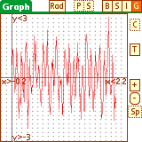
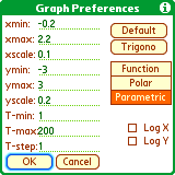

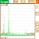
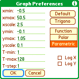

Note the peaks in the spectrum at 5 and 12 Hz.
Back to Contents
Normal matrix addition, subtraction, and multiplication are supported.
Examples:
matrix_q+matrix_p
a-[[0:0]:[1:-1]]
a*b
identity(n) - returns the n x n identity matrix
matrix_q^-1 - returns the matrix inverse of (user-defined) 'matrix_q'
a' - returns the transpose of matrix 'a'
det(a) - returns the determinant of matrix 'a'
rref(a) - returns the reduced row-echelon form of a matrix. Often used to find a solution to system of equations.
Example with two linear equations:
1x + 2y = 3
4x + 5y = 6
Store the system as an augmented matrix to 'matrix_a':
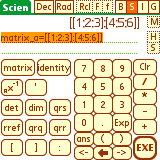
matrix_a=[[1:2:3]:[4:5:6]]
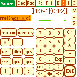
rref(matrix_a)
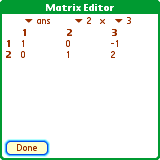
ans> [[1:0:-1]:[0:1:2]]
The solution is found in the right column of the answer (x=-1, y=2).
EasyCalc can factor a matrix 'a' into matrices qrq(a) and qrr(a). qrr(a) generally decomposes a full rank matrix to a simpler form.
For an m x n matrix:
q=qrq(a) returns an orthogonal m x m matrix
r=qrr(a) returns an upper triangular m x n matrix
The result of qrq(a) * qrr(a) is the original matrix 'a'.
Example:
mat3_4=[[1:2:3:4]:[2:3:4:5]:[3:4:5:6]]
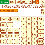
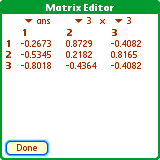
q=qrq(mat3_4)
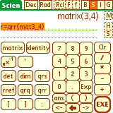
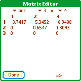
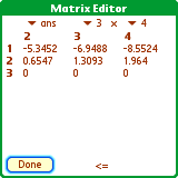
r=qrr(mat3_4)
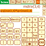

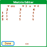
qrq(mat3_4) * qrr(mat3_4)
ans> [[1:2:3:4]:[2:3:4:5]:[3:4:5:6]] (the original matrix)
Linear systems in the form 'Ax = b' can be solved by replacing 'A' with 'QR'. qrs(Ab) uses Householder QR decomposition and back-substitution. This approach may solve matrices that are not solvable with rref().
Example:
matrix_a=[[1:2:3]:[4:5:6]]
qrs(matrix_a)
ans>[[1:2:-1]:[4:5:2]]
The original 'A' matrix is returned, augmented with the solution 'x',
which is (-1, 2).
Note: for qrs(), matrices can be complex, but the 'A' matrix part must currently be square.
To find the eigenvalues of a matrix, find the zeros of:
evalue()="det(x(2)-(x(1))*identity(sum(dim(x(2))*[1:0])))"
Example:
a=[[1:3]:[2:2]]
graph -> "evalue(x:a)" - gives zeroes (Eigenvalues) at -1 and 4.
Back to Contents
npr(n:r) - permutations of n obj taken r at a time
ncr(n:r) - n Choose r for combinations (the Binomial Coefficient)
Examples:
npr(8:3)
ans> 336
ncr(8:3)
ans>56
gamma(x)
The 'Q' notation is taken from the Handbook of Mathematical Functions,
edited by Abramowitz and Stegun. This reference is also credited with
many of the formulas that permit the leveraging of other functions
already included in EasyCalc.
EasyCalc uses the lngamma function. This permits
the use of large numbers for the degrees of freedom of several of the
probability functions.
The Upper-Tail Probability functions return 1 minus the Cumulative
Distribution Function (CDF). You must compute '1-qFunction' to get the
Lower-Tail Probability.
qBinomial(c:n:p) - returns the probability of more than 'c' successes,
given the number of trials 'n', and probability of success 'p'.
Where: {0 <= c, n>0, 0 <= p <= 1}
qBeta(x:a:b) - returns the probability of getting a value greater than
'x', given the Beta coefficients 'a' and 'b'.
Where: {0 <= x <= 1, a>0, b>0}
qChiSq(ChiSq:df) - returns the probability of getting a value greater
than 'ChiSq', given 'df' degrees of freedom.
Where:{0 <= ChiSq, df>0}
qF(F:df1:df2) - returns the probability of getting an F-ratio value
greater than 'F', given numerator and denominator degrees of freedom
'df1' and 'df2'.
Where: {F=>1, df1>0, df2>0}
qPoisson(c:lam) - returns the probability of getting more than 'c'
occurrences, given the occurrence rate of 'lam'.
Where: {0 <= c, 0 <= lam}
qStudentt(t:df) - returns the probability of getting a t-ratio greater
than 't', given 'df' degrees of freedom.
Where: {0 <= df}
qWeibull(t:a:b) - returns the probability of getting a value greater
than 't', given scale parameter 'a' and shape parameter 'b'.
Where: {0 <= t, 0 <= b}
qNormal(z) - returns the probability of getting a value greater than 'z' for the standard normal distribution with mean 0 and standard deviation 1.
Example: Compute 90% Confidence Interval:
For the standard normal distribution the 90% confidence interval for the
mean 0 lies between -1.645 and +1.645. Here we compute it for a normal
distribution with mean 100 and standard deviation 10:
xbar=100
s=10
z90=1.645
xbar+z90*[-1:1]*s
ans> [83.6:116.4]
Back to Contents
All functions and operations can take complex arguments (if allowed mathematically).
Complex numbers are represented as '4+5i' ('i' or 'j' indicates the
complex part). When a complex number is stored in 'ans', the 'M' menu
offers to convert to '->e^(ix)' or '->c()+isin()' format:
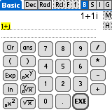
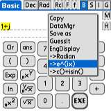
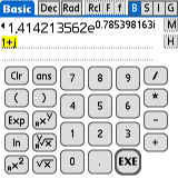
1+j
ans> 1+i
M ->e^(ix)
ans> 1.414213562e^(0.785398163i)
M ->GuessIt
ans> sqrt(2)e^pi*i/4
M ->c()+isin()
ans> 1.414213562(cos(0.785398163)+i*sin(0.785398163))
The functions specific to complex numbers are:
real(x) - real part of number:
real(2+3i)
ans> 2
imag(x) - imaginary part of number:
imag(2+3i)
ans> 3
conj(x) - complex conjugate:
conj(2+3i)
ans> (2-3i)
or
(2+3i)'
ans> 2-3i
abs(x) - absolute value:
abs(3+4i)
ans> 5
angle - angle of complex vector to the real axis:
{in radian mode}
angle(1+i)
ans> 0.785 398 163
M ->Radian
ans> 0.25pi
M ->GuessIt
ans> pi/4
Back to Contents
Switch to the Integer form by tapping 'I' at the top of the main screen. Then, check 'Force integer nums' in the Preferences. (If you leave this unchecked, numbers will be treated as 'float'. Binary operations are not defined for floating point numbers.)
- Select the original base.
- Enter a value or expression. Note that you must press "EXE" to get the
value stored in ANS before converting.
- Select the base to convert to.
Example (on Integer form):
{tap 'Dec' button}
1234{EXE}
ans> 1,234
{tap 'Bin' button}
ans> 100,1101,0010
{tap 'Oct' buttin}
ans> 2322
{tap 'Hex' button}
ans> 4D2
-EA ...{ans-EA displayed}
ans> 3E8
{tap 'Dec' button}
ans> 1,000
EasyCalc works with 32-bit integers and supports simple
bit-wise binary operations:
x & y - x AND y
x | y - x OR y
x ¥ y - x XOR y (the 'yen' symbol)
x << n - logical shift left n bits
x >> n - logical shift right n bits
Note: When leaving Integer mode, don't forget to uncheck 'Force integer nums' in the Preferences. It will cause unexpected errors and truncated results outside of Integer mode. Also, you will usually want to set Dec mode again.
factor(a) - return a list of prime factors of a
factor(12)
ans> [2:2:3]
gcd(a[:b:c:...]) - greatest common divisor
gcd(10:14:12)
ans> 2
lcm(a[:b:c:...]) - lowest common multiple
lcm(10:12)
ans> 60
gcdex(a:b) - returns a list of cofactors (x and y so that
a*x+b*y=gcd(a,b)) and gcd and lcm
gcdex(14:10)
ans> [14:-2:10:3:2:70]
means gcd=2, lcm=70 and 14*-2+10*3=2
modinv(a:b) - computes inverse of a modulo b, i.e. the number x with
0 <= x < b and (a * x) % b == 1
modinv(2:17)
ans> 9
since (2 * 9) % 17 = 18 % 17 = 1
modpow(a:b:c) - computes (a ^ b) % c, but will not cause any rounding
errors if a < c < 65536
modpow(5:50:10000)
ans> 5625
since 5 ^ 50 = 88817841970012523233890533447265625. However, when computing
(5^50)%10000 directly you get 3440.
phi(a) - computes the totient (Euler's phi function) of a,
i.e. the number of positive integers less than or equal to a and
coprime to a
phi(666)
ans> 216
chinese(a1:n1:a2:n2:[a3:n3:...])
- computes the solution of the Chinese remainder theorem. Every pair of
parameters (ai, ni) means
x % ni == ai, the resulting x will solve all equations.
The ni must be coprime (may not have common factors)
chinese(42:100:2:3)
ans> 242
isprime(a) - returns 1 if a is prime, 0 otherwise
isprime(17)
ans> 1
nextprime(a) - returns the smallest prime larger or equal to a
nextprime(200)
ans> 211
nextprime(97)
ans> 97
prevprime(a) - returns the largest prime smaller or equal to a
prevprime(200)
ans> 199
prevprime(97)
ans> 97
Back to Contents
EasyCalc can find approximate numeric (not symbolic) solutions to equations on an interval. These functions are also available from the Graph layout. You may find that to be an easier interface, and it allows you to better specify the interval. Try to specify a small interval (min and max close together). If you receive the error 'Impossible Calculation', you may need to adjust the interval and/or the error tolerance, or there may be no solution.
The following parameters are used in this section:
min - left bound of interval
max - right bound of interval
func - a literal expression enclosed in double quotes such as
"x^3-x^2-5", or a user defined function such as f()="x^2-4".
The first parameter must be "x", additional parameters are x(2), x(3), etc.
Example: "x^2-3x+2*x(2)-x(3)+1"
error - The maximum error tolerance allowed in the answer. Defaults
to 1E-10. The smaller the error, the longer the computation time.
{:params} - additional parameters passed to x(2), x(3), etc. if the
function has multiple variables.
fzero(min:max:func{:error{:params}}) - This function finds a root
(may not be unique!) of a function using the 'division of interval'
method.
In the following examples, we change the interval and error tolerance (the
exact roots are -2, -1 and 1):
fzero(-10:10:"x^3+2x^2-x-2")
ans> 1.000 000 001
fzero(-10:10:"x^3+2x^2-x-2":1E-2)
ans> 1.000 976 563
fzero(-10:0:"x^3+2x^2-x-2")
ans> -1.999 999 997
The following example sets up the general quadratic function a*x^2 + b*x
+ c, sets values for the coefficients, an passes those as parameters
into fzero().
quad()="x(2)*x^2+x(3)*x+x(4)"
a=2;b=3;c=-2
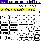
fzero(-100:100:quad():1E-8:a:b:c)
ans> -1.999 999 999
fvalue(min:max:value:func{:error{:params}}) - finds a point where f(x)=value
fmin(min:max:func{:error}) - finds the minimum of the function in the interval [min,max]
fmax(min:max:func{:error}) - finds the maximum of the function in the interval [min,max]
fintersect(min:max:f1:f2{:error{:params}}) - finds a point where f1(x)=f2(x) .
fd_dx(x:func{:error{:params}}) - finds the first derivative of the
function at the point 'x'.
fd2_dx(x:func{:error{:params}}) - finds the second derivative at the
point 'x'.
Examples:
fd_dx(3:"x^3+2x^2-x-2")
ans> 38
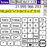
fd2_dx(3:"x^3+2x^2-x-2":1E-6)
ans> 21.999 966 293
EasyCalc can approximate integrals using Simpson's Rule:
fsimps(min:max:func{:error{:params}})
Example:
fsimps(0:pi:"sin(x)")
ans> 2
fsimps(0:1:"x+x(2)":1E-6:1)
ans> 1.5
or by Romberg Integration (usually better):
fromberg(min:max:func{:degree{:params}})
degree - an optional integer parameter that specifies the degree of the
polynomial used to approximate the function.
Computation time can become very long for large values of "n" (more than
n=10 or so -
fromberg(0:pi:"sin(x)":15) takes about 120 seconds on a Palm M500.).
Example:
fromberg(0:pi:"sin(x)")
ans> 2
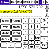
fromberg(0:pi:"sin(x)":3)
ans> 1.998 570 732
Back to Contents
The EasyCalc Solver (found in the Special Menu) uses the fzero() function to find numeric solutions of multi-variable equations.
To use the Solver:
Tap the 'down triangle' and select 'New Worksheet'. Name the worksheet.

On the two dashed lines, enter an equation (WITHOUT double-quotes), such
as: s=1/2*a*t^2.
Finish with the 'Update' button (or the Graffiti 'Return' stroke).
The box will list the variables used in the expression, and their
current values.
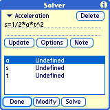
Tap a variable and tap 'Modify' (or double-tap) to change its value.
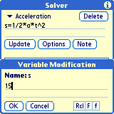
Select a variable and tap 'Solve' to solve the equation for that variable. If you enter an expression without an equals sign, you can tap 'Calculate' to evaluate the expression with the current variable values.
'Note' button
Tap 'Note' to add a short description of each variable. Enter the
description after the colon on the note form. This description is then
displayed in the main Solver form when you select that variable.
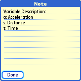
'Options' button
Tapping 'Options' allows you change the following:
Name: The worksheet name
Minimum/Maximum: The interval to search for a solution on.
Precision: The maximum error tolerance allowed in the solution.
These values are passed into the fzero() function.

Back to Contents
Time Value of Money (TVM) Calculation (Ordinary Annuities)
You can calculate the mortgages, loans, savings, and investments using EasyCalc's TVM Calculator.
I - Annual Interest Rate (in percent)
N - Total Number of Payments
PV - Present Value
PMT - Payment (Annuity)
FV - Future Value
P/YR - Number of Payment Periods per Year
Begin/End - Payment made at the beginning or end of the period
(normally END).
Tapping the Value (the right side) lets you change the value of the
variable.
Tapping the Variable Name (the left column) solves for that variable.
This implementation uses the "cash flow" meaning of sign. "+" can be taken as money to the bank, and "-" as money from the bank.
Example:
What are my monthly payments on a $20,000, five-year auto loan at 8% APR?
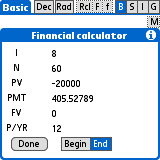
Tap the right column to enter these values:
I - 8
N - 60
PV - -20000 (Remember '-' means from the bank)
PMT - undefined
FV - 0
P/YR - 12
Begin/End - END
Tap PMT in the left column to calculate the monthly payment: $405.53.
Change the interest rate to "6", and tap PMT again to see the payment
drop to: $386.66
Back to Contents
Most functions/operators can take scalar, list, matrix, or complex operators (if the operation makes sense).
pi 3.141592653589793
e 2.718281828459045
euler 0.577215664901533
i,j sqrt(-1)
x default parameter in functions
ans result of previous operation
m milli- prefix (1E3 EngDisplay)
u micro- prefix (1E-6 EngDisplay)
n nano- prefix (1E-9 EngDisplay)
p pico- prefix (1E-12 EngDisplay)
f femto- prefix (1E-15 EngDisplay)
k kilo- prefix (1E3 EngDisplay)
M mega- prefix (1E6 EngDisplay)
G giga- prefix (1E9 EngDisplay)
T tera- prefix (1E12 EngDisplay)
+ addition
- subtraction, unary minus
* multiplication
/ division
^ exponentiation
x%y x modulo y (remainder)
= variable/function assignment
x<<n shift x left 'n' bits
x>>n shift x right 'n' bits
& bit-wise logical AND
| bit-wise logical OR
¥ (YEN) bit-wise logical XOR
, alternate decimal point
; separates expressions on a single line
Arithmetic Comparisons (return 1 if true, 0 if false)
== equality
>= greater than or equal to
<= less than or equal to
d°m's deg°min'sec angle notation
a' matrix transpose of matrix 'a'
c' complex conjugate of scalar 'c'
[:] matrix/list delimiters
() parens for expression collection
f()="expr" define function 'f'
exp(x) power of e to the x
ln(x) natural logarithm
log(x) logarithm base 10
log2(x) logarithm base 2
sqrt(x) square root
cbrt(x) cube root
abs(x) absolute value
neg(x) arithmetic negation
floor(x) next integer <= x
ceil(x) next integer >= x
round(x{:dec}) rounds x up or down to 'dec' decimal places
trunc(x{:dec}) discards fractional part of x past 'dec' decimal places
ipart(x{:dec}) same as trunc(x{:dec})
fpart(x) fractional part of x
fact(x) x factorial
real(x) real part of a number
imag(x) imag. part of a number
angle(x) angle of complex number to real axis
conj(x) complex conjugate of x
sign(x) -1 if neg, 1 if pos, 0 if 0
int(x) convert float to integer
factor(a) - return a list of prime factors of a.
gcd(a[:b:c:...]) - greatest common divisor.
lcm(a[:b:c:...]) - lowest common multiple.
gcdex(a:b) - returns a list of cofactors (x and y so that
a*x+b*y=gcd(a,b)) and gcd and lcm.
modinv(a:b) - computes inverse of a modulo b, i.e. the number x with
0 <= x < b and (a * x) % b == 1.
modpow(a:b:c) - computes (a ^ b) % c, but will not cause any rounding
errors if a < c < 65536.
phi(a) - computes the totient (Euler's phi function) of a.
chinese(a1:n1:a2:n2:[a3:n3:...])
- computes the solution of the Chinese remainder theorem.
isprime(a) - returns 1 if a is prime, 0 otherwise.
nextprime(a) - returns the smallest prime larger or equal to a.
prevprime(a) - returns the largest prime smaller or equal to a.
sin(x)
cos(x)
tan(x)
asin(x)
acos(x)
atan(x)
atan2(y:x) = atan(y/x)
sinh(x)
cosh(x)
tanh(x)
asinh(x)
acosh(x)
atanh(x)
Back to Contents
list(elem{:elems}) - list of elements
matrix(m:n:elem{:elems}) - m x n matrix of elements
dim(mat_x) - size of list/ matrix "mat_x" [m:n]
sift(f:x) - drops all elements for which f returns zero<.br />
sift(x:y) - drops all elements from y where x is zero.
find(f:x) - returns indices where f(x) is nonzero.
sample(x:y) - returns the elements of x indexed by y.
map(f:x) - applies f to each element of x.
map(f:x:y) - applies f to each pair of x and y (not only
matching pairs).
zip(f:x:y) - applies f to each maching pair of x and y.
concat(x:y) - concatenates two lists.
repeat(x:a:b) - will repeat a list's elements. a means how
often to repeat, b means how large parts (0 for full list) to repeat.
kron(x:y) - computes all possible products between the elements
of x and those of y.
det(mat_x) - determinant of matrix 'mat_x'
rref(mat_x) - reduced row echelon form of matrix 'mat_x'
identity(n) - n x n identity matrix
cmatrix(m:n:{elements}) - m x n matrix of complex elements
qrq(mat_x) - QR factorization, quotient
qrr(mat_x) - QR factorization, remainder
qrs(mat_x) - solution using QR factorization.
rtopr(x:y) - rectangular to polar Radius
rtopd(x:y) - rectangular to polar Angle
rtop(x:y) - rectangular to polar (returns a list [radius:angle])
ptorx(rad:ang) -polar to rectangular x-coord
ptory(rad:ang) -polar to rectangular y-coord
ptor(rad:ang) - polar to rectangular (returns a list [x:y])
hypot(x:y) - length of the hypotenuse of a right triangle with sides
x and y.
I = annual interest
N = total number of payments
PV = present value
PMT = payment
FV = future value
P/YR = payments/year
flag=0 end of month payment
flag=1 beginning of month payment
fin_pv(I:N:PMT:FV:PYR:flag)
fin_n(I:PV:PMT:FV:PYR:flag)
fin_fv(I:N:PV:PMT:PYR:flag)
fin_pmt(I:N:PV:FV:PYR:flag)
fzero(min:max:func{:error{:params}})
fmin(min:max:func{:error})
fmax(min:max:func{:error})
fvalue(min:max:value:func{:error{:params}})
fintersect(min:max:f1:f2{:error{:params}})
fd_dx(x:func{:error{:params}})
fd2_dx(x:func{:error{:params}})
fsimps(min:max:func{:error{:params}})
fromberg(min:max:func{:degree{:params}})
npr(n:r) - r permutations of n
ncr(n:r) - n Choose r (combinations)
qBinomial(c:n:p) - probability of > 'c' successes with 'n' trials,
'p' probability of success
qBeta(x:a:b) - probability of > 'x', with Beta coefficients
'a' & 'b'
qChiSq(ChiSq:df) - probability of > 'ChiSq' with 'df' degrees
of freedom
qF(F:df1:df2) - probability of F-ratio > 'F' with numerator and
denominator degrees of freedom 'df1' and 'df2'
qPoisson(c:lam) - probability of > 'c' occurrences with occurrence
rate of 'lam'
qStudentt(t:df) - probability of t-ratio > 't' with 'df' degrees
of freedom.
qWeibull(t:a:b) - probability of value > 't' with scale parameter 'a'
and shape parameter 'b'
qNormal(z) - probability of value > than 'z'
mean(listx) - arithmetic mean of listx
lmin(listx) - min value of listx
lmax(listx) - max value of listx
sum(listx) - sum of elements of listx
median(listx) - median of listx
sorta(listx) - ascending sort of listx
sortd(listx) - descending sort of listx
gmean(listx) - geometric mean of listx
prod(listx) - product of elements of listx
variance(listx{:flag}) - variance of listx; if flag==0, uses unbiased
'sample' formula; if flag==1, uses 'population' formula
stddev(listx{:flag}) - standard deviation of listx; if flag==0, uses
unbiased 'sample' formula; if flag==1, uses 'population' formula
skewness(listx) - skewness of list
kurtosis(listx) - kurtosis of list
varcoef(listx) - coefficient of variance of listx
cumsum(listx) - returns a list containing the cumulative sums of the
elements of listx
lmode(listx) - most frequently occurring element in listx
moment(listx:n) - n'th moment of listx
cov(listx,listy) - covariance of listx and listy
corr(listx,listy) - correlation coefficient of listx and listy
linreg(listx,listy) - linear regression of listx and listy
randseed(x) - (reproducibly) starts the pseudo-random series
rand - uniform random num from 0..1
rand(n) - list of 'n' uniformly rand elements
rNorm(n)- list of 'n' normally distributed random elements, mean=0,
stddev=1
range(n{:start{:step}}) - returns an n-dimension list containing sequential values.
Back to Contents
filter(x:a:b) - filters the data in vector x with the filter
described by vectors a and b.
conv(x:y) - convolution of two signals.
dft(x[:N]) - N-point Discrete Fourier Transform of a signal.
idft(x[:N]) - N-point Inverse Discrete Fourier Transform.
fft(x[:N]) - N-point Fast Fourier Transform of a signal.
ifft(x[:N]) - N-point Inverse Fast Fourier Transform.
fftshift(x) - shift DC component to center of spectrum.
euler - 0.577215664901533
gamma(z) - Euler Gamma Function
beta(z:w) - Beta Function
igamma(a:x) - Incomplete Gamma Function
ibeta(a:b:x) - Incomplete Beta Function
erf(x) - Error Function
erfc(x) - Complementary Error Function
besselj(n:x) - Bessel Function 1st Kind
bessely(n:x) - Bessel Function 2nd Kind
besseli(n:x) - Modified Bessel Function 1st Kind
besselk(n:x) - Modified Bessel Function 2nd Kind
ellc1(m) - Complete Elliptic Integral 1st Kind
ellc2(m) - Complete Elliptic Integral 2nd Kind
elli1(m:phi) - Incomplete Elliptic Integral 1st Kind
elli2(m:phi) - Incomplete Elliptic Integral 2nd Kind
sn(m:u) - Jacobi Elliptic Function sn
cn(m:u) - Jacobi Elliptic Function cn
dn(m:u) - Jacobi Elliptic Function dn
todeg(x) - display as D°M'S
todeg2(x) - display as D°m.sss
torad(x) - display as n*pi
togonio(x) - display as c()+isin()
tocis(x) - display as e^(ix)
ask("title"{:default value}) - opens a dialog with the (optional)
default entered. Returns the user input.
if(test:"expr if true":"expr if false") - evaluates test and returns
the appropriate expression. Test must return a positive integer ('true') or
zero ('false' ).
unset(name) - clears function or variable 'name' from memory
defparamn(x) - DO NOT USE. Sets the parameter name to
something other than 'x'. Some functions (e.q. most of the q<something>
statistical functions) are defined internally as strings using 'x' as the
parameter name. They will not work if you change the parameter name !!!
Back to Contents
Can be copied and pasted into EasyCalc.
Speed of light in vacuum (m s-1)
c=299792458
Newtonian constant of gravitation (m3 kg-1 s-2)
g=6.67259E-11
Standard gravitational acc. (kg)
g=9.80665
Electron mass (kg)
me=9.1093897E-31
Proton mass (kg)
mp=1.6726231E-27
Neutron mass (kg)
mn=1.6749286E-27
Atomic mass unit (unified) (10-19 C)
u=1.6605402E-27
Electron charge (J s)
q=1.60217733E-19
Planck constant (J K-1)
h=6.6260755E-34
Boltzmann constant (H m-1)
k0=1.380658E-23
Magnetic permeability (F m-1)
u0=1.2566370614E-6
Dielectric permittivity (m)
e0=8.854187817E-12
Classical electron radius (none)
re=2.81794092E-15
Fine structure constant (m)
al=0.00729735308
Bohr radius (m-1)
a0=5.29177249E-11
Rydberg constant (Wb)
r=10973731.53
Fluxoid quantum (J T-1)
fq=2.06783461E-15
Bohr magneton (J T-1)
ub=9.2740154E-24
Electron magnetic moment (J T-1)
ue=9.2847701E-24
Nuclear magneton (J T-1)
un=5.0507866E-27
Proton magnetic moment (J T-1)
up=1.41060761E-26
Neutron magnetic moment (m)
un=9.6623707E-27
Compton wavelength (electron) (m)
lc=2.42631058E-12
Compton wavelength (proton) (W m-2 K-4)
lcp=1.32141002E-15
Stefan-Boltzmann constant (mol-1)
sig=5.67051E-8
Avogadro's constant (mol-1)
na=6.0221367E+23
Ideal gas volume at STP (J mol-1 K-1)
vm=0.0224141
Universal gas constant (C mol-1)
r=8.31451
Faraday constant (Ohm)
f=96485.309
Quantum Hall resistance (m3 kg-1 s-2)
rh=25812.8056
Back to Contents
Scientific Calculator for PalmOS.
Copyright (C) 1999 - 2003, 2006, 2007 Ondrej Palkovsky
This program is free software; you can redistribute it and/or modify it under the terms of the GNU General Public License as published by the Free Software Foundation; either version 2 of the License, or (at your option) any later version.
This program is distributed in the hope that it will be useful, but WITHOUT ANY WARRANTY; without even the implied warranty of MERCHANTABILITY or FITNESS FOR A PARTICULAR PURPOSE. See the GNU General Public License for more details.
You should have received a copy of the GNU General Public License along with this program; if not, write to the Free Software Foundation, Inc., 51 Franklin Street, Fifth Floor, Boston, MA 02110-1301, USA.
You can contact the developers via the Open Discussion Forum http://sourceforge.net/forum/forum.php?forum_id=41375 on the project website http://sourceforge.net/projects/easycalc
Back to Contents
Main author: Ondrej Palkovsky (ondrap at penguin.cz)
I send many thanks to these people and others for contributing to this
project, many of the features that you are using wouldn't exist without
their help.
Rafael R. Sevilla (dido at pacific.net.ph)
Added many mathematical functions and improved the old code.
Richard Scott (rts4377 at yahoo.com)
Contributed the Upper Tail probabilities, romberg integration code,
improvements of special functions
Jorge Gil (cluny at users.sourceforge.net)
Michael Schierl (schierlm at users.sourceforge.net)
Recent inprovemens of code since 1.23
John Hodapp (bigshot at email.msn.com)
Code improvements regarding matrices, UI etc.
Ton van Overbeek (ton at v-overbeek.nl)
PalmOS5 compatibility, hires and DIA patches. Recent releases.
Edgar Piskernik (pisker at gmx.at)
Harald Lueling (Harald_Lueling at burg-waechter.de)
German translation
Francesco (fcroci at prodigy.net.mx)
Spanish translation
Carlos Irapuan Lube de Menezes (cirapuan at hotmail.com)
Portuguese translation
Daniel Lemire, Ph.D. (lemire at ondelette.com)
French translation
Ignazio Di Napoli (neclepsio at hotmail.com)
Michele Mazzucchi (m.mazzucchi at linuxpratico.com)
Italian translation
Yoshimov (yoshimov at pobox.com)
Japanese translation
Pavel Kharitonov (dti17 at narod.ru)
Russian translation
Olga Yiparaki (yiparaki at mindspring.com)
Sent me utilities for matrix functions
Antonio Fiol Bonn_n (Antonio.FIOL at enst-bretagne.fr>
Added PYR support for the financial equations
Koichi Takagi (halliday at users.sourceforge.net)
Updated documentation
For more information about the GNU General Public License: http://www.gnu.org/copyleft/gpl.html
For more information about the MathLib library: http://www.radiks.net/~rhuebner/mathlib.html
Back to Contents