Now to some of the things you can see
on screen. The 'Rcl' is for fast access to variables, 'F' is for fast access to
functions (be sure and create your own - see below) and 'H' stands for
history.
There are 2 different layouts of the Basic screen. You can switch it
in Preferences. The second form of the Basic layout is more crowded,
but some people like it.

You can use the solver to store and document your formulas. If there is no '='
found, Solver just computes the result.

It is possible to add additional parameters to the function being solved.
All parameters that are passed to fzero() after the error parameter
are passed to the inner function.
a=[[1:2]:[3:4]]
b=[[5:6]:[7:8]]
a+b


Identity matrix generation
identity(n)
This function generates an identity matix with dimension n.
Example: identity(3)

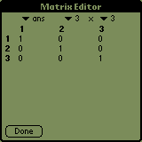
You get the answer matrix(3,3). This means that the matrix is too large to be
displayd on the result line. Tap the result to see the matrix in matrix editor, you will
find the identity matrix:

Matrix inversion and transposition
(matrix_a)^(-1)
(matrix_a)'
Example:
a=[[1:2]:[3:4]]
a^(-1)


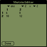
You can find the result matrix under the variable ans:

To check the correct answer you can multiply matrix a with matrix ans
with the result of [[1:0]:[0:1]] which is a unit matrix.
Example:
a=[[1:2:3]:[4:5:6]]
b=a'


The resulting b matrix is:

Matrix reduction operation
rref(a)
This functions reduces dependent rows, it is usually used to find
a solution to system of equations.
Example:
1x + 2y =
3
4x + 5y =
6
Put these two linear equations in matrix form with right hand side
appended as right column.
a=[[1:2:3]:[4:5:6]]
rref(a)
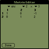
A row echelon form is returned as evidenced by
the leading 1's propagating downward and to the right.
The results for x and y are returned as the right column of
rref(a). And the solution can be
verified, see below.
1*(-1) + 2*(2) = 3
4*(-1) + 5*(2) = 6


Matrix QR Factorization
qrq(a) and
qrr(a) return Q and R respectively as Factorization of
matrix a
qrs(Ab) solves linear equation Ax = b like rref
only using QR decomposition and backsubstitution. This
approach may
solve matrix that are not solvable with rref.
The qrq and qrs functions combined will compute the orthogonal Q, and upper
triangular R matrix, respectively, of an m x n matrix using Householder
method. For m = n, Q and R are the same size as the original
matrix. For m(rows) x n(cols) the Q matrix is size m x m and R is
size m x n. The result of qrq(a) * qrr(a) should return the original
matrix ' a '. QR generally decomposes a full rank matrix to a simpler
form.
Another interesting property is that Q*Q' =
Q'*Q = I the
identity matrix.
Examples:
First enter a matrix --- ' mat3_4=[[1:2:3:4]:[2:3:4:5]:[3:4:5:6]]
'
then try --- ' qrq(mat3_4) '
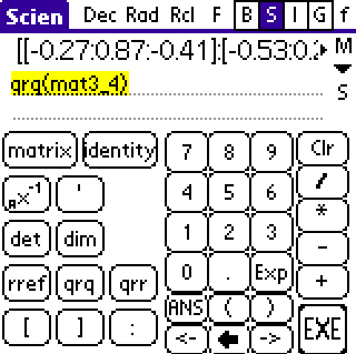
 Q
Q
and ' qrr(mat3_4) '
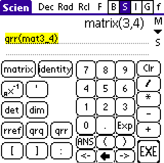
 R - upper triangular - but zero is near
1e-16.
finally try ' qrq(mat3_4) * qrr(mat3_4)
'
 The original matrix - use => to see remaining columns.
Given Q and R, problems such as Ax = b can readily be solved by
replacing A with QR. This is readily accomplished with
function qrs.
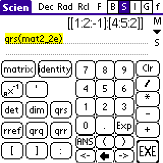
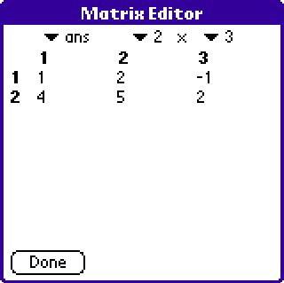
In this example the same matrix a appended with b as used
above for rref was entered into mat2_2e. The original a
is returned along with
the solution x which is -1, 2. Note: The Matrix can be
complex but also note that for qrs the matrix must currently
be square.
Other matrix functions
- det(a) - determinant of a
matrix
- dim(a) - returns list of 2 values where first value is number of rows and second is number of columns
Integer functions
- factor(a) - return a list of prime factors of a: factor(12) = [2:2:3]
- gcd(a[:b:c:...]) - greatest common divisor: gcd(10:14:12) = 2
- lcm(a[:b:c:...]) - lowest common multiple: lcm(10:12) = 60
- gcdex(a:b) returns a list of cofactors (x and y so that a*x+b*y=gcd(a,b))and gcd and lcm: gcdex(14:10) = [14:-2:10:3:2:70] - means gcd=2, lcm=70 and 14*-2+10*3=2
- modinv(a:b) computes inverse of a modulo b, i.e. the number x with 0 <= x < b and (a * x) % b == 1: modinv(2:17)=9 since (2 * 9) % 17 = 18 % 17 = 1
- modpow(a:b:c) computes (a ^ b) % c, but will not cause any rounding errors if a < c < 65536: modpow(5:50:10000) = 5625 since 5 ^ 50 = 88817841970012523233890533447265625. (5^50)%10000 = 3440, however.
- phi(a) computes the totient (Euler's phi function) of a, i.e. the number of positive integers less than or equal to a and coprime to a: phi(666) = 216
- chinese(a1:n1:a2:n2:[a3:n3:...]) computes the solution of the Chinese remainder theorem. Every pair of parameters (ai, ni) means x % ni == ai, the resulting x will solve all equations. The ni must be coprime (may not have common factors). chinese(42:100:2:3)=242.
- isprime(a) returns 1 if a is prime, 0 otherwise: isprime(17) = 1
- nextprime(a) returns the smallest prime larger or equal to a: nextprime(200) = 211. nextprime(97) = 97
- prevprime(a) returns the largest prime smaller or equal to a: prevprime(200) = 199. prevprime(97) = 97
Preferences
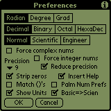
- Radian/Degree/Grad mode change - this change applies to all functions.
- Decimal/Binary/Octal/Hexadecimal - this setting applies to output formatting
- Force integer input -
this setting applies to input recognition
and displaying functions, but doesn't change computing behavior. This means,
that expression '3.14159' isn't recognized in non-floating modes,
because '3.141..' is a floating point number, while 'pi' outputs the correct
result regardless of mode, because 'pi' is a floating point constant.
Generally you do not want to turn this option on, unless you want to work
with base conversions, because floating point output formatting prints at
most 10 digits, but the integer number formatting will print always the
whole number (this makes sense only for 32-bit numbers converted to Binary).
- Strip zeros - output '3.100' or '3.1'
- Match ()'s - if on, then tapping the function button automatically
inserts the closing bracket and moves the cursor position between the brackets
- Force complex nums - because complex operations are slow and usually
less precise, all computation are done as 'real' by default. This doesn't
at all confine you in the real sphere, because the calculator automatically
switches to complex operations whenever it encounters complex numbers.
- Reduce precision - personally I don't like things like sin(pi)=1E-15.
This is unfortunately the way most computers work and I can't do much about
it, it is the limitation of floating point. If this is checked, EasyCalc
rounds numbers after every operations to 11 places
respecting floating point number representation and makes results
of certain functions smaller then 1E-14 equal to zero. Selecting this option
slows all operations a little, that's why I recommmend switching it off if you
are going to use Function Solving (if you are using function solving from
graphs, reduce precision turns off automatically).
- Show units - If checked and the engineer mode is selected, numbers get
appended a unit to them at the output (e.g. 1E6 -> 1M ).
- Basic=>Scien - Allows you to choose between 2 layouts of the Basic
screen - either really basic or more scientific.
- Palm Num Prefs - If checked, EasyCalc allows entering
numbers exactly according to PalmOS Preferences. I do not recommend setting it
unless you use clipboard for moving data from other applications.
Integer calculations
Tap the
' I ' on the top and change to the 'Integer' screen:
 In
this example enter 'ABCDEF' with HEX selected then select BIN.
EasyCalc works with 32-bit unsigned integers and supports simple binary
operations - AND(&), OR(|), ShiftLeft(<), ShiftRitght(>) and
XOR(the 'yen'). It
also supports base conversions. If you do not check the
Integer input in preferences, all numbers will be treated as 'float' and for
float numbers are not defined the and,or,shl and shr operations. Write in some number and press the 'Exe' key and the number will
appear in the Result area. Now tap on the base you want to convert to and the
number will be converted. DO NOT FORGET TO CHECK THE MODE BACK TO DECIMAL AND
UNCHECK THE INTEGER INPUT, you can be surprised to see BAD results if you do not
(3/2 in integer is not the same as 3/2 in floating point). BTW: If the result is
longer than the result field, a small arrow appears on the right and you can
scroll the field by touching the field and moving with the pen left/right.
Complex calculations

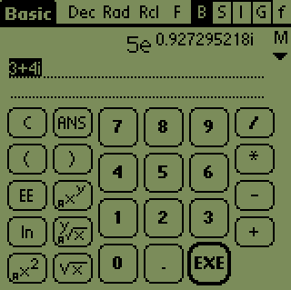
EasyCalc supports
all ordinary computations with complex numbers (please, write me
if you find some operation EasyCalc doesn't support, it is possible I forgot
some of them). The 'i' works exactly as expected. On the second figure you
see the result of number conversion in the 'M' menu ' ->e^(ix) ' . The functions
specific to complex numbers are:
- real - real part of number: real(2+i) = 2
- imag - imaginary part of number: imag(2+i) = 1
- conj or apostrophe: conj(2+i) = (2+i)' = (2-i)
- abs - absolute value: abs(3+4i) = 5
- angle - angle(1+i) = pi/4
Variables and functions
EasyCalc supports an unlimited number of variables and functions.
Variable (or function) names consist of lower-case letters and
can be up to 10 characters long. Variables and functions share the same
address space, so if you define a variable with the same name as a function, the
function will be overwritten. Variable is defined simply by executing
'name=value', a function is defined by executing 'name()="code"'. The 'name'
cannot be 'pi', 'e' and 'x' as these are reserved identifiers.
And now some examples: writing a=31 and
tapping the Exe key will assign a number
31 into variable a. From now you can treat the variable a like
other constants. If you now write a=3*a, variable a will contain
the number 93.
Let's try to define a simple function now: write f()="x^2" and press
Exe. From now you can use this a function - f(3) will return a
result of 9. You can easily delete/modify all defined functions and
variables by tapping the 'DataMgr' in the 'M'-menu on the right of the result
field.
You can define your own functions that accept more then 1 parameter. You have
to call the second parameter as x(2) third as x(3) etc. E.g.
f()="x(1)+x(2)".
Financial calculator
Introduction to financial calculations
Basic financial calculation can be characterized this way:
You have some money in the bank (PV, present value). X-times a year(P/YR,
payments per year) you deposit some money (PMT, payment) into your bank
account. Every year the Bank adds some amount of money, a percentage of
the amount that is currently on your account. The percentage is called
interest (IT).
After a given number of years (NP, Number of deposits) you decide to withdraw
your money from the bank. What you will get from bank is a future value(FV).
End of introduction
This is a basic implementation of financial calculator. You work with 6
different variables:
IT - interest pr. year. Note: from the 1.01 version this should be a
per-cent number, e.g. 12% interest should be written as i=12 and not as
i=0.12, like in earlier versions.
NP - number of payment-periods
PV - present value
PMT - payment (annuity) every period
FV - future value
P/YR - payments per year
and the Begin/End buttons, that affect when is the payment done - in the
beginning of the year or at the end (usually at the end).
Now you can try defining 5 variables and by tapping on the name of the 6th
it gets computed. Let's try an example:
By tapping on the buttons 'Undefined' near names of corresponding variables
you can enter values for every variable. Now most of those
'Undefined' messages should have disappeared. If you tap on the name of the
variable you wanted to compute, a notice 'Please wait' will appear in the
middle of the screen
indicating, that the calculator is computing, and you'll be able to
read the result as soon as the sign disappears.
Graphs
EasyCalc can display functions as a graph.It currently supports normal
function graphs, polar and parametric graphs.
Let's begin with drawing a simple graph. Go to graph preferences
(tap 'G' and then the letter 'P' or 'menu->Graph->preferences') and set it
exactly as you can see it on the screen-shot.

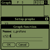
Now exit the preferences and go to setup (tap 'S' or 'menu->Graph->Setup
funcs'). Tap the blank space on the right of 'Y1' and enter "x^2-4". Exit setup
and look at the graph. If you see the graph to be drawing too fast,
you can make it faster by tapping the 'Sp' button and choosing the speed.
For the higher speed you get lower quality though.
If you want to delete a function or graph an already existing one, tap on
the function identifier (Y1,r1...) and a popup menu appears. Select 'None'
to hide a function, 'User' to create a special function for this graph (the
same one, as when you tap to the right of the identifier) or choose an
already existing function.
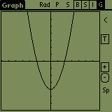
What can you do with the graph screen? If you tap on the graph and move the
pen, the
graph moves too. After you lift the pen, the graph is redrawn. The '-' button
is for 'zoom out' and the '+' button is for 'zoom in' (press the '+' button
and draw a rectangle, where do you want the new screen to be).
If you want to read the graph values, go to Menu->graph->table mode, and
what you read are values of the parameter (x) and values of f(x).

You may want to trace a function like in the older version of EasyCalc. Tap
the 'T' on the right, select a function and tap on the screen. This works
perfectly for normal functions, but works somewhat worse for Polar and
doesn't work at all for Parametric functions. That's why you can use up/down
arrows and/or the 'Go' button to draw a cross directly on some value. You
may also start typing the value directly by graffiti and the 'GoTo' window
appears automatically.

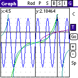
 Parametric 'Art' ?
EasyCalc can do some numerical mathematics, it can compute root, minimum and
maximum of a function, first and second derivation and integral. Tap the 'C'
button on on the right side of screen and follow instructions. Result of the
computation will be stored in a variable called 'graphres'.
 Selected 'C' and minimum then set left and right
boundaries ...
Lists
EasyCalc can do some operations with lists of numbers. Lists with complex
numbers are allowed although some operation do not work with them. You can
define lists either with the List Editor or on command line. I belive the List
Editor is easy to use, only if you want to append an item to the list, select
some item in the list and start writing numbers, input window appears and
the number will be added to the list.
Lists can be thought as an extension of computation engine of EasyCalc. Most
normal operation accept lists and produce a list as a result. E.g.
sin(list(0:pi/2:pi)) = list(0:1:0). Of course you can freely add, subtract,
multiply lists. The variation of a list can be easily defined as:
sum(x-sum(x)/ldim(x))/ldim(x) (and it will work with complex numbers).
Lists work with these functions:
- list(a[:b:c:...]) - creates a new list: list(1:2:3)=[1:2:3]
- range(n[:start[:step]) - creates an n-dimension list containing sequential values: sample(5:0:2)=[0:2:4:6:8]
- sum(x) - computes total sum of the list: sum(list(i:1:2)) = 3+i
- mean(x) - computes mean of the list: mean(list(1:2:3)) = 2
- gmean(x) - computes geometrical mean of the list: gmean(list(1:2:4)) = 2
- median(x) - computes median of the list: median(list(3:2:5)) = 3
- sorta(x),sortd(x) - sorts the list using absolute value of every item:
sort(list(4:2:5)) = list(2:4:5)
- prod(x) - computes total product of the list: prod(1:2:3) = 6
- min(x),max(x) - finds minimum/maximum in the list
- dim(x) - number of items in list: ldim(1:2:3) = 3
- lmode(x) - most frequently occuring item in a list: lmode(1:2:3:3) = 3
- variance(x[:flag]),stddev(x[:flag]) - computes variance (or standard deviation)
using sum(x-mean(x))/(ldim(x)-1). If flag is set to nonzero value,
computes variance using sum(x-mean(x))/ldim(x).
Standard deviation is defined as sqrt(variance()).
- moment(x:n) - computes an n'th moment of a list
- skewness(x), kurtosis(x), varcoef(x) - computes skewness, kurtosis and coefficient of
variance
- cov(x:y), corr(x:y) - computes covariance and
correlation coefficient of lists
- sift(f:x) - drops all elements for which f returns zero: sift("x<9":list(2:9:3:10:1)) = list(2:3:1). sift("isprime(x)":range(100) returns list of primes.
- sift(x:y) - drops all elements from y where x is zero, both lists must have same length: sift(list(1:2:0:1):list(9:2:3:9)) = list(9:2:9).
- find(f:x) - returns indices where f(x) is nonzero: find("isprime(x)":[10:11:12:13:14]) = [2:4] since 11 and 13 are prime.
- sample(x:y) - returns the elements of x indexed by y: sample([0:1:2:3:4]:[1:3:5])=[0:2:4]
- map(f:x) - applies f to each element of x. In most cases this is done transparently (map("x+1":[3:4]) = [3:4] + 1, but in some cases not. map("a[x]":list(3:1)) will return list(a[3]:a[1])
- map(f:x:y) - applies f to each pair of x and y (not only matching pairs): map("x(1)+x(2)":[2:5]:[10:30]) = [12:15:32:35]
- zip(f:x:y) - applies f to each maching pair of x and y: zip("x(1)+x(2)":[2:5]:[10:30]) = [12:35]
- concat(x:y) - concatenates two lists: concat([1:2]:[3:4:5]) = [1:2:3:4:5]
- repeat(x:a:b) - will repeat a list's elements. a means how often to repeat, b means how large parts (0 for full list) to repeat: repeat([1:2:3:4]:3:0) = [1:2:3:4:1:2:3:4:1:2:3:4], repeat([1:2:3:4]:3:1) = [1:1:1:2:2:2:3:3:3:4:4:4], repeat([1:2:3:4]:3:2) = [1:2:1:2:1:2:3:4:3:4:3:4], repeat([1:2:3:4]:3:3) = [1:2:3:1:2:3:1:2:3:4:4:4]
- kron(x:y) - computes all possible products between the elements of x and those of y: kron([1:2:3:4]:[1:0:-1])=[1:0:-1:2:0:-2:3:0:-3:4:0:-4]
Digital Signal Processing
- filter(x:a:b) - filters the data in vector x with the filter described by vectors a and b to create the filtered data y. The filter is an implementation of the standard difference equation: a(1)*y(n)=b(1)*x(n)+b(2)*x(n-1)+...+b(nb+1)*x(n-nb)-a(2)*y(n-1)-...-a(na+1)*y(n-na)
- conv(x:y) - convolution of two signals. (If x and y are vectors of polynomial coefficients, convolving them is equivalent to multiplying the two polynomials)
- dft(x[:N]) - N-point Discrete Fourier Transform of a signal.
- idft(x[:N]) - N-point Inverse Discrete Fourier Transform.
- fft(x[:N]) - N-point Fast Fourier Transform of a signal. (N is a power of 2)
- ifft(x[:N]) - N-point Inverse Fast Fourier Transform. (N is a power of 2)
- fftshift(x) - shift DC component to center of spectrum.
(CAUTION: dft and idft are very slow procedures, they can hold your device for a long time with large values of N. Use fft and ifft instead)
Hints
- If you have selected text on screen and tap a function button (e.g. sin,
but a plain '(' would do), the selected text will be inserted into the
function.
- Remember that you can still use the on-screen keyboard anytime you need
to input numbers. This is very handy in the 'GoTo' dialog when you are
tracing function.
- You may experience strange results when graphing functions do not have
some values defined, e.g. tan(x) when you zoom-out. There is no way I can
fix it if I do not want to make it considerably slower. You can make it
slower yourself, when you draw this as a parametric graph (set 'X=x' and
'Y=tan(x)'. Then you can choose the T-step small enough to let the graph
draw exactly as you expected..
- EasyCalc can guess a number. Suppose you just computed 'acos(0)' and you
don't know what the result means. Use the M->GuessIt and it will tell
you, that you just got 'pi/2'. When guessing an integer number, prime
factors are shown.
- If you want to go to the certain value in Graph Table
mode, just start typing the new value, you do not have to tap the 'GoTo'
button. The same goes for tracing the function.
Function Reference
- % - modulo operator: 10 % 3 = 1
- the 'yen' character - xor
- ask("Question"[:default]) - Asks the question and expects user input.
If you are in graph mode, the user is not asked and the 'default' is
provided instead. If there is no default, you get an error.
- fact(x) - computes factorial: fact(5) = 120
- ncr(x:y) - combination: ncr(5:3) = 10
- npr(x:y) - permutation(?): npr(5:3) = 60
- rand - random number: rand = 0.548020875
- ipart(x),trunc(x) - the whole part of a number,
accepts one optional parameter - number of dot points: ipart(1.52:1) =
trunc(1.52:1) = 1.5
- round(x) - round a number, takes optional second parameter as trunc(): round(3.7) = 4
- sign(x) - x>0 -> 1, x<0 -> -1, x==0 -> 0. sign(-4) = -1
- floor(x) - largest integral value not greater than x: floor(-1.5) = 2
- fpart(x): fpart(2.3) = 0.3
- hypot(y:x) - sqrt(x^2+y^2): hypot(3:4) = 5
- atan2(y:x) - phase angle: atan2(1:1) = pi/4
- EasyCalc with special functions supports these functions: gamma(z),
beta(z:w), igamma(a:x), erf(x), erfc(x), ibeta(a:b:x), besselj(n:x),
bessely(n:x), besseli(n:x), besselk(n:x), elli1(m:phi), elli2(m:phi),
ellc1(m), ellc2(m), sn(m:u), cn(m:u), dn(m:u). If you want additional help,
please look in specfuncs.pdf that is included with the installation.
- defparamn("x") - allows you to set the parameter name
to something other than 'x'. DO NOT USE IT AS IT CAN BREAK SOME INTERNAL CODE
(some internal code including some functions depends on this variable to be
set to 'x'. You can safely change this parameter in definition manager,
because it affects only the defined function).
Contact, Newest information etc.
It might be useful to read documents you get with EasyCalc, especially
'INSTALL'.
EasyCalc was written by Ondrej Palkovsky,
ondrap@penguin.cz. Latest
information is available on
http://easycalc.sourceforge.net.
I send many thanks to people who reported bugs and sent me language
corrections to this tutorial. This product is still changing and if you feel
that you encountered a bug (including an error in this tutorial, english is
not my first tongue) feel free to contact me.


 enter '3+3' EXE ->


 . But
only, of course, if you learn how to write the special degree character, or
select the Basic=>Scien check box in Preferences to get a Basic screen that
has the degree and minute characters (right hand figure above). The
Degree/Radian/Grad can be switched in Preferences or as a convenience you can
change the mode by tapping the Deg/Rad/Grd indicator at the top of the
display. Selection of Dec/Hex/Oct/Bin can be made in the same way.
This saves time in that you do not need to go to Preferences Screen to change
trig modes or number radix.


 You get the answer 21.


 where the
derivative is
  . Let x=2, then
 .
.


 Q
Q
 R - upper triangular - but zero is near
1e-16.
 The original matrix - use => to see remaining columns.


 In
this example enter 'ABCDEF' with HEX selected then select BIN.


 Parametric 'Art' ?
 Selected 'C' and minimum then set left and right
boundaries ...